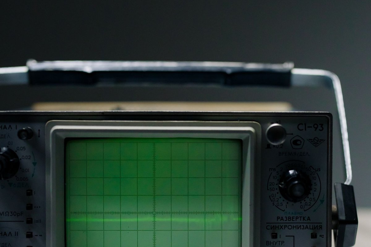
FMCW radar is one of the most widely used radar architectures in short- and medium-range sensing. The letters stand for frequency-modulated continuous wave, which describes exactly what the transmitter does: it keeps radiating a signal without pause, and it changes the frequency of that signal over time in a controlled, repeating pattern.
That simple idea has big consequences. Because an FMCW radar measures targets by comparing frequencies rather than timing separated pulses, it can deliver very fine range resolution with modest transmit power, see objects at extremely short distances, and estimate range and velocity in the same measurement chain. These properties make FMCW a natural fit for automotive sensing, industrial level measurement, presence detection, and — increasingly — low-altitude security and counter-drone surveillance.
This article explains how FMCW radar works from the ground up: the chirp, the beat frequency, the processing chain, the numbers that define performance, and the limitations that engineers have to design around.
The Core Idea: Transmit Continuously, Sweep the Frequency
A basic pulse radar behaves like someone shouting in a canyon: it sends a short burst of energy, goes quiet, and measures how long the echo takes to come back. The time delay multiplied by the speed of light gives the distance.
An FMCW radar never goes quiet. Instead, it transmits a continuous signal whose frequency ramps upward (or downward) in a straight line over a short interval. One such ramp is called a chirp, and the radar repeats chirps in a rapid, regular sequence. A single chirp might sweep across a few hundred megahertz in tens of microseconds, although real designs vary widely.
The receiver listens while the transmitter is still on. When an echo from a target arrives, the radar does not ask “how long did this take?” directly. Instead it asks “how different is the frequency coming back from the frequency I am transmitting right now?” That frequency difference carries the range information, because the echo is simply a delayed copy of the chirp, and a delayed copy of a linear ramp is offset in frequency by an amount proportional to the delay.
How a Chirp Becomes a Distance
The key mechanism is the beat frequency. When the received echo is mixed with a sample of the currently transmitted signal, the mixer outputs a low-frequency signal whose frequency equals the difference between the two. For a stationary target and a linear chirp, that difference is constant for the duration of the sweep:
- The chirp sweeps bandwidth B over chirp duration T.
- The echo arrives delayed by the round-trip travel time, which equals 2R/c (twice the range divided by the speed of light).
- The beat frequency is therefore proportional to range: fb = (2R/c) × (B/T).
The processing chain measures that beat frequency, and the radar converts it straight back into distance. A target twice as far away produces a beat note exactly twice as high. Multiple targets at different distances each produce their own beat frequency at the same time, and a spectrum analyzer — in practice an FFT running on digitized samples — pulls them apart into separate peaks. Each peak is a target at a different range.
This is the elegant part of FMCW: a continuous high-frequency measurement problem is transformed into a low-frequency one. The beat notes from short-range targets typically fall in the kilohertz to low-megahertz region, which is easy to digitize with ordinary, power-efficient analog-to-digital converters. That is one reason compact FMCW sensors can be built small and affordable.
Measuring Range and Velocity at the Same Time
A moving target shifts every echo by the Doppler effect. In an FMCW radar that Doppler shift appears in two places. Within a single chirp it slightly biases the beat frequency, coupling range and velocity together. Across a sequence of chirps it shows up as a steady phase rotation from one chirp to the next, because the target moved a little between consecutive sweeps.
Practical FMCW radars exploit the second effect. The processor collects a frame of many chirps — often tens or hundreds — and runs a second FFT across them. The first FFT resolves targets in range; the second resolves them in Doppler, which converts directly to radial velocity. The result is a range-Doppler map: a two-dimensional grid in which every detected object appears as a peak with both a distance and a speed.
Simultaneous range and velocity measurement is one of FMCW’s defining strengths. A security radar watching for small drones, for example, does not just need to know that something is there; it needs to separate a slow-moving rotorcraft from stationary clutter such as trees, fences, and buildings. The Doppler dimension provides exactly that separation.
Inside a Typical FMCW Radar
Although implementations differ, most FMCW radars share the same functional blocks:
- Waveform generator. A synthesizer — commonly a phase-locked loop or a digitally controlled source — produces the chirp: a clean, linear frequency ramp repeated at a precise rate. The quality of this ramp (its linearity and phase noise) sets a floor under measurement accuracy.
- Transmit front end. Amplifiers raise the chirp to the required power level and feed the transmit antenna. FMCW radars generally run at low continuous power rather than high peak power.
- Receive front end. A separate receive antenna (or a shared antenna through a duplexer) collects the weak echoes, which low-noise amplifiers boost before mixing.
- Mixer and de-chirping. Mixing the received signal with a copy of the transmitted chirp produces the beat-frequency signal. This step is often called de-chirping or stretch processing.
- Digitizer and FFT processing. An analog-to-digital converter samples the beat signal, and digital logic — an FPGA, DSP, or embedded processor — performs the range FFT, the Doppler FFT, detection, and tracking.
Because all of these blocks operate continuously at modest power, they integrate well onto compact RF chips and small circuit boards. That integration is why FMCW dominates in cost- and size-sensitive sensing markets.
The Numbers That Define an FMCW Radar
A handful of parameters describe what any FMCW radar can do. Understanding them makes datasheets much easier to read.
Sweep bandwidth (B) sets range resolution — the minimum spacing at which two targets can still be told apart. The relationship is fundamental: resolution equals the speed of light divided by twice the bandwidth (ΔR = c / 2B). A 150 MHz sweep resolves targets about one meter apart; 300 MHz resolves about half a meter; 1 GHz reaches roughly fifteen centimeters. Bandwidth, not transmit power, is what lets an FMCW radar separate a drone from the wall behind it.
Chirp duration (T) influences how much energy is collected per sweep and how large the Doppler-induced error in the beat frequency becomes. Longer chirps gather more energy but couple range and velocity more strongly; shorter chirps reduce that coupling but demand faster, wider-bandwidth electronics.
Chirp repetition rate and frame length determine how often the radar refreshes its picture and how finely it resolves velocity. More chirps per frame mean finer Doppler resolution and better separation of slow movers from clutter, at the cost of a slower update or more processing.
Transmit power and antenna gain set the power budget, which — together with target reflectivity — limits maximum detection range. FMCW radars typically transmit milliwatts to a few watts continuously rather than kilowatt-class pulses.
Update rate is how many full measurements per second the system delivers. Security and tracking applications usually want updates fast enough to build smooth tracks on maneuvering targets.
Why FMCW Works Well for Short-Range, Low, Slow, and Small Targets
Several FMCW properties line up almost perfectly with the problem of detecting low, slow, small objects — the classic profile of hobby-class drones and similar low-altitude targets.
First, there is effectively no close-in blind range caused by transmit timing. A pulse radar cannot receive while its high-power pulse is being transmitted, which creates a minimum-range dead zone. An FMCW radar receives continuously, so targets a few meters away are measurable as long as the hardware keeps the transmitter’s leakage under control.
Second, fine range resolution comes from bandwidth, not power. Small objects close to clutter — a drone near a tree line, for instance — can be separated in the range dimension even when the echoes are weak. High resolution also shrinks the amount of clutter competing inside each resolution cell, which improves the signal-to-clutter ratio for small targets.
Third, continuous low-power transmission is easy to integrate, runs cool, and is practical for fixed sites, vehicles, and mast-mounted security sensors. Low peak power also simplifies power supplies and thermal design.
Finally, the built-in range-Doppler processing separates slow movers from stationary backgrounds, which is exactly what low-altitude surveillance needs when the environment is full of static structures, vegetation, and ground clutter.
FMCW and Pulse Radar: The Short Comparison
The full FMCW-versus-pulse discussion deserves its own article, and this site has one — see FMCW vs Pulse Radar: Advantages and Limitations Explained for the detailed comparison and What Is Pulse Doppler Radar? for the pulsed side of the story. The beginner summary is short:
- Pulse radar measures the time of flight of separated bursts and typically uses high peak power, which scales well to long-range surveillance.
- FMCW radar measures the frequency offset of a continuous swept signal and typically uses low continuous power, which scales well to compact short- and medium-range sensing.
Neither is universally better. The choice follows the mission: range, resolution, size, power, and cost all push the decision one way or the other.
Limitations and Engineering Trade-offs
FMCW radar is not free of weaknesses, and honest evaluation matters more than enthusiasm. Three limitations come up in almost every design discussion.
Long-range power budget. Because transmit power is low and continuous, the energy on a distant, weakly reflecting target is limited. Stretching detection range usually means larger antennas, more integration time, or higher transmit power — each of which erodes the size and cost advantages. For long-range surveillance, pulsed architectures often remain the more natural fit.
Transmitter-to-receiver leakage. The transmitter never switches off, so some of its energy inevitably couples directly into the receiver through the antenna arrangement, cabling, or nearby reflections. That leakage appears as a huge signal at or near zero range and can mask real targets or saturate the receiver if isolation is poor. Antenna separation, careful layout, and digital cancellation techniques all exist to manage it, but leakage control is one of the hardest practical problems in FMCW design and a major reason cheap sensors underperform their paper specifications.
Dense multi-target scenes. Each target creates a beat peak per chirp, and with simple single-ramp waveforms the range-Doppler coupling can make it ambiguous which peaks belong to which object. Multi-chirp patterns, varied slopes, and tracking logic resolve most of this, but in genuinely crowded environments — many birds, vehicles, and drones at once — association and ghost suppression cost real processing effort.
Interference between neighboring radars and non-linearity in the chirp generator are further concerns that sit behind the resolution and accuracy numbers on a datasheet.
Where FMCW Fits in Low-Altitude Security and Counter-UAS
In the low-altitude security world, a short-range FMCW security radar typically plays the role of the always-on detection layer: it scans a volume around a site, produces range-Doppler detections, and hands tracks to classification logic, cameras, or other sensors. Its strengths — fine range resolution, good slow-target Doppler sensitivity, no close-in dead zone, and compact low-power hardware — match the mission of watching for small drones approaching at low altitude over cluttered terrain.
The same characteristics explain FMCW’s role beyond security: automotive parking and blind-spot sensing, tank level gauging, industrial presence detection, and robotics all rely on the same chirp-and-beat-frequency principle at even shorter ranges.
The important framing is that waveform choice is only one layer of system performance. Antenna design, processing quality, installation height, site clutter, and integration with other sensors shape real-world outcomes just as much as the modulation format printed in the brochure.
Practical Takeaways
FMCW radar is best understood as a frequency-comparison instrument. It transmits a continuously sweeping chirp, mixes the echo with what it is currently sending, and reads distance off the resulting beat frequency while reading velocity off the phase progression across chirps. Sweep bandwidth sets range resolution, chirp timing shapes Doppler behavior, and the continuous low-power architecture delivers compact hardware with excellent short-range performance.
Its trade-offs are equally definable: limited long-range power budget, the constant fight against transmitter leakage, and processing complexity in crowded target scenes. For short-range, low-altitude, small-target sensing — including counter-drone surveillance — those trade-offs usually land in FMCW’s favor, which is why the architecture has become a default building block in that mission space.
Further Reading
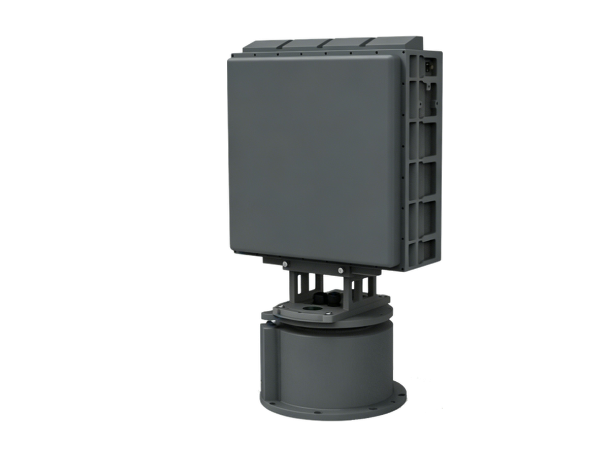
Need Counter-Drone Radar for Your Site?
CR series low-altitude surveillance radars detect RCS 0.01 m² drones at 3–10 km and classify targets by micro-Doppler — every track outputs with target class and confidence.