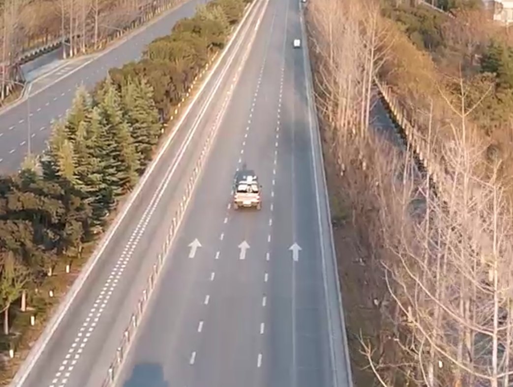
A counter-drone radar that only works while parked leaves a gap exactly where mobile units need protection most. Convoys, patrol vessels, mobile border posts, and rapid-response teams all share the same problem: the moment they move, a conventional surveillance radar either goes blind or drowns in self-induced clutter. Radar on the move — usually abbreviated OTM (on the move) — is the engineering answer: a radar that continues to detect, track, and classify low-altitude targets while the platform underneath it is driving, sailing, or maneuvering.
This article is a technical walkthrough of how OTM capability is actually implemented on a four-faced phased array radar. We will look at why platform motion breaks radar physics, how a GNSS/INS inertial navigation module restores it, how the compensation chain is organized across FPGA and GPU processors, what performance the fixed-site four-faced family delivers as the baseline for a mobile configuration, and how motion compensation is validated in theory and practice. Whether you are evaluating a vehicle-mounted counter-UAS radar or designing a mobile low-altitude surveillance concept, this is the vocabulary and the mental model you need.
Why Platform Motion Breaks Conventional Radar
A pulse-Doppler radar measures targets by comparing the phase of successive echoes. Anything that disturbs that phase relationship degrades detection. A moving platform disturbs it in three distinct ways.
First, own-motion Doppler shift contaminates the clutter spectrum. When the radar itself moves, every stationary object on the ground — buildings, terrain, vegetation, fences — acquires an apparent radial velocity relative to the sensor. Instead of clustering around zero Doppler, ground clutter smears across a range of Doppler frequencies that depends on the platform’s speed and the look direction of each beam. Slow targets such as hovering or low-flying drones, which normally stand out precisely because their Doppler differs from stationary ground, are now buried inside a moving clutter ridge. This phenomenon is called clutter migration, and it is the single biggest reason a stationary-tuned radar fails on a vehicle.
Second, attitude changes corrupt beam pointing. A vehicle pitching over rough ground or a vessel rolling in swell constantly changes the orientation of the antenna reference frame. A beam that was supposed to illuminate 5° elevation may actually point at 3° or 7°. Coverage gaps open and close rhythmically, monopulse angle measurements inherit the platform’s angular motion, and the declared elevation coverage on the datasheet stops describing reality.
Third, measured target velocity is no longer ground-relative. The Doppler the radar measures is the relative radial velocity between sensor and target. To know whether a contact is a drone closing on the convoy or a stationary pole receding behind it, the platform’s own velocity vector must be subtracted from every measurement — continuously, for every beam direction.
All three problems share one root cause and, conveniently, one cure: the radar needs an accurate, real-time answer to the question “how am I moving right now?” — and must fold that answer into beam steering and signal processing on every coherent processing interval.
The Motion Reference: GNSS/INS Integrated Navigation
The enabling component of an OTM radar is a GNSS/INS integrated navigation module — a satellite receiver fused with an inertial measurement unit (IMU). Mounted rigidly inside the radar assembly, it continuously outputs the platform’s full motion state:
- Three-dimensional velocity vector in the navigation frame (east–north–up, ENU), so the processor knows exactly how fast the sensor is translating in every direction;
- Complete attitude angles — pitch, roll, and yaw — so the processor knows how the antenna frame is tilted and headed at every instant;
- High-precision position (latitude, longitude, altitude), which anchors tracks to the map and lets the operator see where contacts are in absolute terms, not just relative to a moving sensor.
The satellite and inertial channels complement each other. GNSS provides drift-free absolute velocity and position, but at modest update rates and with vulnerability to obstruction; the IMU provides high-rate angular and acceleration data that bridges GNSS gaps and captures fast attitude dynamics, at the cost of integration drift. The fused output is smooth, fast, and absolute — exactly what real-time compensation needs.
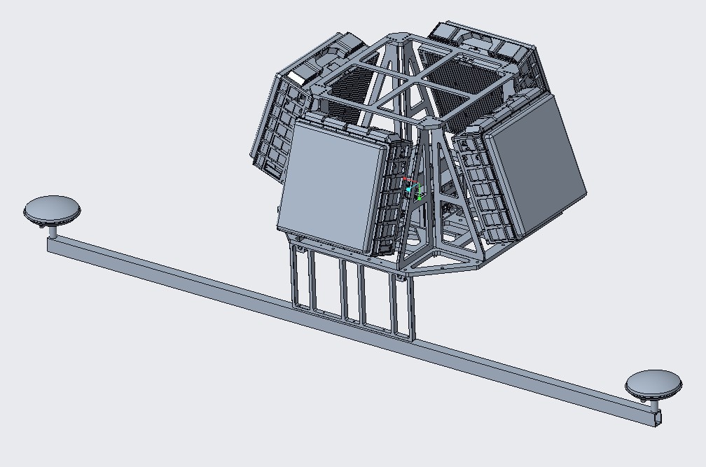
One mechanical detail matters enormously here: the four antenna panels and the fusion module containing the GNSS/INS are rigidly connected by a metal bracket, so the angular rates and accelerations measured by the IMU genuinely represent the motion of the antenna apertures. Any flex or backlash between the IMU and the panels would appear as uncompensated beam jitter. OTM performance is therefore as much a structural-engineering property as a signal-processing one.
System Architecture of an OTM Four-Faced Array Radar
An OTM-configured four-faced array radar consists of four major elements: the antenna panels, the integrated control module (which hosts the GNSS/INS), the power module, and the GNSS antennas.
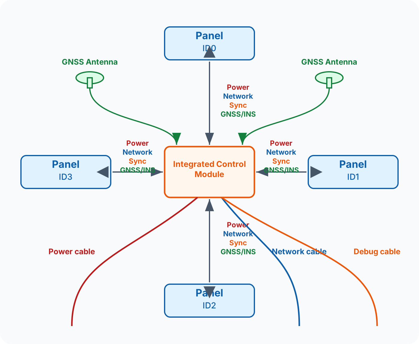
Each of the four panels covers a 90° azimuth sector, giving instantaneous 360° coverage with no mechanical rotation — an essential property for OTM, as we will see. Every panel receives four services from the integrated control module over a combined cable: power (24 V distribution), network (gigabit Ethernet for control and target data), synchronization (so all four panels transmit and receive in a coherent time base), and the GNSS/INS data stream. Externally, the module connects to the platform’s power supply, to the operator console over a single network cable, and to a debug interface for maintenance.
The integrated control module is the system’s traffic hub. Its processing board carries out five functions that make four panels behave as one radar:
- Power distribution — it takes the 24 V input and feeds all four panels from a single point;
- System synchronization — it generates the timing reference that keeps the panels coherent with each other;
- Communications — it receives control parameters from the operator console and distributes them to each panel;
- Inter-panel track fusion — it merges the per-panel target tracks into one seamless 360° track picture for the display, so a drone crossing a panel boundary never becomes a new contact;
- Navigation data distribution — because all four panels share one GNSS/INS, the board broadcasts the motion state to every panel’s signal processor, where it feeds the attitude-stabilization, beam-pointing, and Doppler-compensation algorithms.
Inside the Panel: From Antenna Element to Signal Processor
Each panel is a self-contained active phased array. Zooming into one panel shows the classic AESA chain, plus the motion-data interfaces that make it OTM-capable.
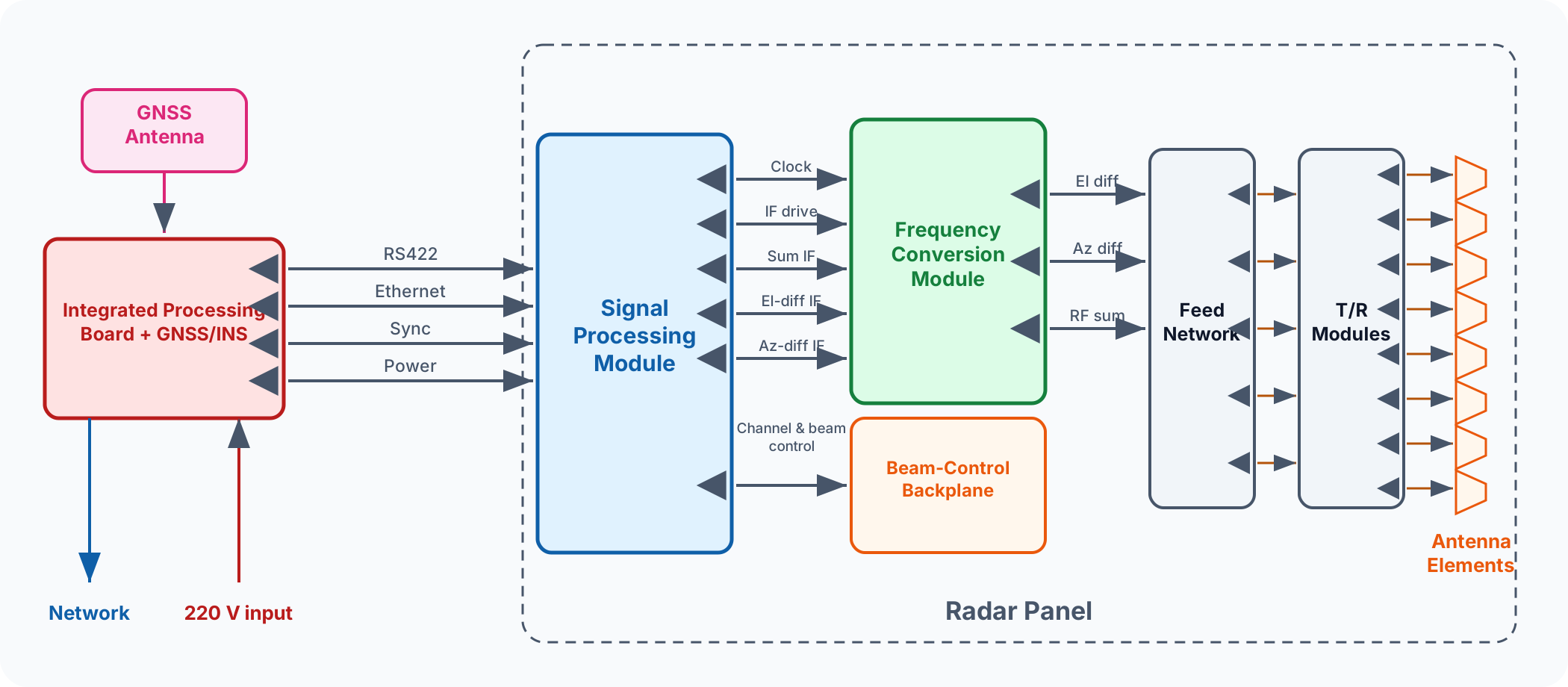
The antenna elements radiate through T/R modules (transmit/receive), which handle power amplification on transmit and low-noise amplification on receive under the control of the beam-control backplane. The feed network combines the element signals into the sum and difference channels (azimuth-difference and elevation-difference) that monopulse angle estimation requires. The frequency conversion module translates between RF and intermediate frequency in both directions. Finally, the signal processing module generates the transmit waveform, digitizes the sum and difference IF channels, and executes the entire detection chain — including, critically, the motion compensation.
Note the interfaces on the left of the diagram: the panel’s signal processor receives RS422 and Ethernet connections to the integrated processing board, the synchronization signal, and power. The navigation data that drives compensation arrives through this path, broadcast from the single shared GNSS/INS. There is no per-panel inertial sensor — one high-quality motion reference, rigidly mounted, serves the whole array. This keeps the four panels referenced to the same motion solution, which is what allows their measurements to be fused into a single coherent track picture afterwards.
The Motion-Compensation Chain: FPGA and GPU Working Together
Compensation is not one algorithm but a pipeline, and it lives where modern radar puts everything else: in software-defined digital hardware. The processing chain is split between an FPGA (for deterministic, sample-rate tasks) and a GPU (for throughput-heavy batch processing).
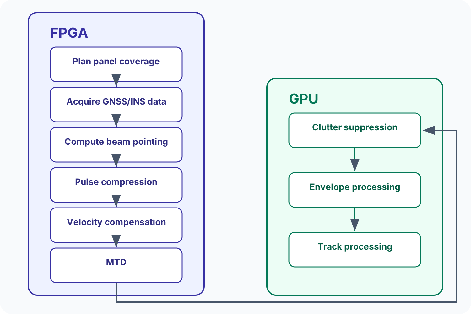
Walking the chain stage by stage:
1. Coverage planning. The mission software defines which azimuth/elevation region each panel must cover — the elevation extent, range scale, and update rate are all software-configurable, so a convoy profile (long range forward, emphasis on low elevations) can differ from a vessel profile.
2. Navigation data acquisition. The processor ingests the current motion state from the GNSS/INS stream: ENU velocity vector, pitch/roll/yaw, and position, time-stamped so compensation applies to exactly the right coherent interval.
3. Beam-pointing computation. Using the instantaneous attitude, the processor recomputes the phase settings for every beam so that beams point where the Earth says they should, not where the tilting platform would put them. This is attitude stabilization in its electronic form: the array’s beam steering absorbs platform pitch and roll in real time, keeping the declared elevation coverage intact while the vehicle rocks. Monopulse angle measurements are likewise rotated back into the stable reference frame.
4. Pulse compression. Received echoes are match-filtered to recover range resolution — identical to fixed-site operation.
5. Velocity compensation. This is the OTM-specific heart of the chain. For every beam direction, the processor computes the platform’s radial velocity along that beam’s line of sight and applies the opposite phase rotation to the received samples. The effect on the data is dramatic: ground clutter, which platform motion had smeared across the Doppler spectrum, is shifted back to where it belongs — the zero-Doppler region — while true moving targets retain their genuine ground-relative Doppler signatures. What was a migrating clutter ridge becomes a stationary clutter spike again.
6. MTD (Moving Target Detection). Doppler filtering then separates targets from clutter in the usual way — but now on a compensated spectrum in which the separation actually exists. Without the previous stage, the filter bank would face clutter in the very channels where slow drones live; with it, those channels are clean.
7. Clutter suppression. Residual ground, sea, and weather returns are adaptively suppressed, with the clutter map continuously rebuilt to follow the moving scene.
8. Envelope processing. Detection envelopes are formed and thresholded, producing the raw plots.
9. Track processing. Plots are associated into tracks, filtered, and passed to the fusion function — where the four panels’ pictures merge into one — and onward to the operator display, which plots every contact in true geographic coordinates.
The practical significance of the FPGA+GPU split is upgradeability: because compensation is software, improvements in stabilization models, clutter handling, or classification ship as firmware updates, not hardware retrofits. The radar’s software-defined, modular architecture — moving the heavy data processing onto a high-performance real-time platform — is what makes an OTM variant of a fixed-site radar feasible at all.
Performance Baseline: The Four-Faced Family
OTM is a configuration of the standard four-faced product line rather than a separate product. The mobile variant inherits the detection performance of its fixed-site sibling; motion compensation then works to preserve as much of that performance as possible while the platform moves. The family spans nine models across X and Ku bands, from short-range point defense to long-range wide-area surveillance:
| Model | Band | Drone detection range (RCS 0.01 m²) | Net weight | Power consumption |
|---|---|---|---|---|
| CR-PX10C | X | ≥1.5 km | ≤45 kg | ≤600 W |
| CR-PX15C | X | ≥3 km | ≤55 kg | ≤1100 W |
| CR-PK13C | Ku | ≥3 km | ≤77 kg | ≤1400 W |
| CR-PX07C | X | ≥5 km | ≤80 kg | ≤1400 W |
| CR-PK05C | Ku | ≥5 km | ≤80 kg | ≤1600 W |
| CR-PX08C | X | ≥8 km | ≤90 kg | ≤2500 W |
| CR-PX16C | X | ≥8 km | ≤130 kg | ≤2400 W |
| CR-PK14C | Ku | ≥8 km | ≤120 kg | ≤3500 W |
| CR-PX11C | X | ≥10 km | ≤125 kg | ≤5500 W |
Common to all nine: instantaneous 360° azimuth coverage with 0°–60° elevation (mission-configurable), all-weather pulse-Doppler operation against low, slow, and small targets, TAS tracking with a ≥500-track capacity, AI classification of drones, birds, people, and vehicles based on micro-Doppler and track features, RJ45 gigabit Ethernet output, AC 220 V / DC 24 V power input, −40 °C to +70 °C operating range, and IP66 environmental protection. Weight and power figures are the practical selectors for mobile integration: a light vehicle or mast-mounted trailer will favor the 45–80 kg models, while a patrol vessel or heavy tactical vehicle can carry the 8–10 km class.
Two properties deserve emphasis in the OTM context. First, no rotating parts: a four-faced array has no pedestal whose inertia fights the platform’s motion and no scan period during which compensation must extrapolate — every direction is illuminated continuously, so stabilization applies everywhere, all the time. Second, a single shared motion reference: one GNSS/INS rigidly mounted to the array serves all four panels, so the fused 360° picture is compensated on one consistent motion solution rather than four independent ones.
OTM Verification: What Good Compensation Looks Like
How do you know motion compensation is working? The theory gives a crisp, observable signature — and it is worth understanding before you ever watch a demo, because it tells you what to ask for.
The canonical evidence is the range-Doppler (RD) map, the two-dimensional intensity plot of echo power versus range gate and Doppler channel. Consider a radar driving down a road and looking sideways at the terrain:
- Before compensation, stationary ground clutter does not sit at zero Doppler. Because every patch of ground has a different angle relative to the velocity vector, its apparent radial velocity varies, and the clutter ridge migrates across the Doppler axis into non-zero channels — precisely the channels where a slow drone must be detected. In an uncompensated RD map you see a broad, tilted clutter band, and any weak target near it is unrecoverable.
- After velocity compensation, the platform’s radial motion along each beam has been subtracted. The clutter ridge collapses back onto the zero-Doppler channel, where standard MTD filtering removes it. The compensated RD map shows a narrow clutter spike at zero Doppler — and, standing clear of it, the genuine target peaks, their energy and position unaffected by the correction.
Two theoretical points are worth noting. First, compensation is a phase rotation, not a filter: it moves the whole spectrum back rather than cutting anything out, which is why true targets are preserved — a well-designed chain neither notches nor desensitizes the Doppler region near clutter. Second, compensation quality is bounded by the motion reference: residual attitude error translates directly into residual pointing error, and residual velocity error into residual clutter spreading. This is why the rigid IMU-to-panel mounting and the fused GNSS/INS solution matter, and why “which INS class do you use?” is a legitimate procurement question.
Validation then follows from the theory. A convincing OTM demonstration compares compensated and uncompensated RD maps recorded in the same run; exercises the geometry that stresses compensation hardest — targets flying opposite the platform’s direction of travel (maximum closing Doppler) and with it (minimum relative Doppler, the case most easily swallowed by the clutter ridge); and confirms that tracks hold continuously through platform turns, when the look direction and thus the compensation solution change fastest. If a vendor can show the clutter returning to zero Doppler while a cooperative drone stays tracked through those geometries, the physics is doing what the theory says it should.
Missions: Where OTM Radar Earns Its Place
Convoy and VIP escort. A moving column cannot stop to scan. A four-faced OTM radar on a lead or escort vehicle maintains a continuous low-altitude bubble around the formation, giving seconds-to-minutes of warning against FPV and fixed-wing drones — with the 5 km class offering a practical balance of reach, weight, and power for light tactical vehicles.
Patrol vessels and coastal craft. A vessel in swell is a permanently moving platform even at anchor. Attitude stabilization absorbs roll and pitch, velocity compensation handles own-ship motion and drift, and the IP66-sealed, −40 °C to +70 °C-rated hardware fits the marine environment. Harbor patrol, offshore platform approaches, and riverine security all benefit.
Mobile border and checkpoint units. Border surveillance increasingly needs to reposition along the frontier on short notice. A vehicle-mounted unit that detects during repositioning closes the coverage gaps that appear exactly when a static system is being moved — the moment an adversary would choose.
Event security and rapid response. For temporary deployments around stadiums, summits, or incidents, a drive-up-and-work system that is already effective while maneuvering into position compresses setup time and keeps protection continuous from arrival to departure.
Evaluating an OTM Radar: A Buyer’s Checklist
OTM claims are easy to print and hard to verify. These questions separate engineering reality from brochure language:
- What is the motion reference? Look for an integrated GNSS/INS (not a bare GPS receiver) with the IMU rigidly coupled to the antenna structure. Ask how attitude is distributed to every panel or channel.
- Where does compensation happen? It must be inside the coherent processing chain (before MTD), not a display-side cosmetic. “We filter it in the tracker” is not motion compensation.
- What happens to the clutter spectrum? Ask to see before/after range-Doppler maps from the same moving run. Clutter should return to the zero-Doppler channel with targets preserved.
- Which geometries were tested? Opposite-direction and same-direction target flights, plus platform turns, stress very different parts of the compensation chain.
- Is the architecture software-defined? FPGA/GPU-based processing means compensation algorithms improve via firmware; fixed-hardware implementations age quickly.
- What is inherited from the fixed-site model? OTM should be a configuration of a proven radar, retaining its detection range, track capacity, and classification stack — not a detuned special variant.
- Integration envelope. Weight, power draw, and connector count decide what vehicles or masts can carry the system. A 24 V DC input simplifies vehicle integration considerably.
Frequently Asked Questions
What does “radar on the move” (OTM) mean? It means the radar maintains detection, tracking, and classification performance while its host platform — a vehicle, vessel, or other carrier — is itself moving, rather than requiring the platform to stop and stabilize before operating.
Why can’t a normal fixed-site radar just be bolted onto a truck? Because platform motion smears ground clutter across the Doppler spectrum (clutter migration), tilts beam pointing through attitude changes, and corrupts target velocity measurements. Without GNSS/INS-based motion compensation integrated into the signal processing chain, a fixed-site radar on a vehicle is largely blind to the slow, low targets it was bought to detect.
What is GNSS/INS and why does an OTM radar need it? GNSS/INS is a fused navigation module combining satellite positioning with an inertial measurement unit. It outputs the platform’s 3D velocity, attitude angles (pitch, roll, yaw), and position in real time. The radar’s processor uses this data to stabilize beam pointing electronically and to subtract the platform’s own motion from the Doppler spectrum — the two corrections that make on-the-move detection possible.
Do rotating radars work on moving platforms? Mechanically scanned radars face extra difficulty on the move: the pedestal’s inertia fights platform motion, stabilization requires a servo loop, and each direction is only revisited once per scan period. Fixed four-faced arrays illuminate every direction continuously and stabilize purely in software, which is why they are the preferred OTM architecture.
Does OTM performance equal fixed-site performance? The mobile configuration inherits the detection envelope of its fixed-site sibling, and good compensation preserves the great majority of it. Residual degradation is bounded by the quality of the motion reference and the compensation chain — which is why the class of GNSS/INS and the rigidity of the installation matter.
Which Cyrentis radars support on-the-move deployment? The full four-faced array family — CR-PX10C, CR-PX15C, CR-PK13C, CR-PX07C, CR-PK05C, CR-PX08C, CR-PX16C, CR-PK14C, and CR-PX11C, spanning 1.5 km to 10 km drone-detection classes in X and Ku band — can be delivered in a mobile-platform configuration with GNSS/INS motion compensation.
The Bottom Line
Radar on the move is not a feature checkbox; it is a chain of engineering decisions — a rigid motion reference, attitude-stabilized beam steering, Doppler velocity compensation ahead of MTD, and a software-defined processing platform to host it all. Four-faced array radars are where that chain is easiest to build well, because nothing rotates and every direction is always covered.
If you are planning a convoy-escort, patrol-vessel, or mobile border-surveillance capability, talk to our team about the mobile configuration of the four-faced family, or explore the individual models — from the 1.5 km CR-PX10C to the 10 km CR-PX11C — in our product lineup.
Need Counter-Drone Radar for Your Site?
CR series low-altitude surveillance radars detect RCS 0.01 m² drones at 3–10 km and classify targets by micro-Doppler — every track outputs with target class and confidence.